M18.L03 — Cost Minimisation: The Isocost-Isoquant Approach
Module: Module 18 — Technology, Production, and Profit Maximisation Lesson: L03 of 05 Duration: ~30 minutes Level: Intermediate Provenance: Intermediate Microeconomics with Excel (Barreto) | MIT OCW 14.01 Principles of Microeconomics
Learning Objective
Key Diagram
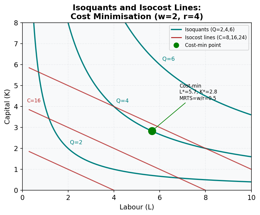
Figure 12: Cost Minimisation. The firm minimises cost at the tangency of the isocost line and isoquant — where MRTS = w/r.
Derive cost-minimizing input combinations using isocost-isoquant tangency.
Cost Minimisation
Given input prices \(w_1\) and \(w_2\), the firm minimizes cost \(C = w_1x_1 + w_2x_2\) subject to producing output \(y\).
Key Concepts:
- Isocost Line: \(w_1x_1 + w_2x_2 = C\). Slope = \(-w_1/w_2\).
- Tangency Condition: MRTS = input price ratio: \(\frac{MP_1}{MP_2} = \frac{w_1}{w_2}\).
- Conditional Factor Demands: \(x_1^*(w_1, w_2, y)\) and \(x_2^*(w_1, w_2, y)\) solve the cost-minimization problem.
- Cost Function: \(C(w_1, w_2, y)\) is the minimized cost.
- Shephard’s Lemma: \(\frac{\partial C}{\partial w_i} = x_i^*\).
Worked Example
[Australian context]
An Australian brewery uses labor (\(x_1\)) and barley (\(x_2\)) with \(y = x_1^{0.5}x_2^{0.5}\). Input prices: \(w_1 = 20\) AUD/hour, \(w_2 = 5\) AUD/kg. 1. Tangency Condition: [ \frac{MP_1}{MP_2} = \frac{x_2}{x_1} = \frac{w_1}{w_2} = 4 \implies x_2 = 4x_1 ] 2. Substitute into Production Function: [ y = x_1^{0.5}(4x_1)^{0.5} = 2x_1 \implies x_1^* = \frac{y}{2}, \quad x_2^* = 2y ] 3. Cost Function: [ C = 20 \left(\frac{y}{2}\right) + 5 (2y) = 20y ]
Common Misconception
"Cost minimization always occurs where MRTS = price ratio."
Only true for interior solutions. Corner solutions (e.g., perfect substitutes) may not satisfy tangency.
Key Takeaways
- Cost minimization requires equating MRTS to input price ratio.
- Shephard’s Lemma links cost function derivatives to conditional factor demands.
- Cobb-Douglas production leads to linear conditional demands in output.
Practice
- For \(y = x_1 + x_2\) and \(w_1 = 2\), \(w_2 = 3\), find cost-minimizing inputs.
- Derive Shephard’s Lemma for \(C = 2w_1^{0.5}w_2^{0.5}y\).
Further Resources
Provenance: Intermediate Microeconomics with Excel (Barreto) | MIT OCW 14.01 Principles of Microeconomics