M15.L01 — The Slutsky Equation: Decomposing Price Effects

Module: Module 15 — Comparative Statics and Demand Theory Lesson: L01 of 05 Duration: ~30 minutes Level: Intermediate Provenance: Intermediate Microeconomics with Excel (Barreto) | MIT OCW 14.01 Principles of Microeconomics

---

Learning Objective

Key Diagram

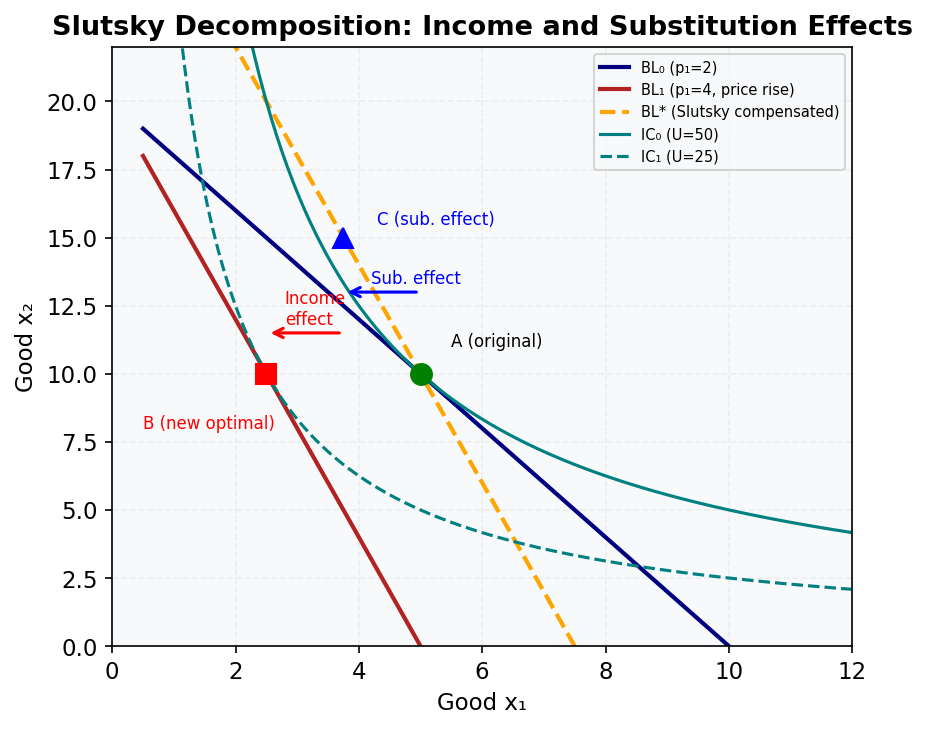
Figure 10: Slutsky Decomposition. A price rise moves the consumer from A to B. The substitution effect (A→C, along the compensated budget line) and income effect (C→B) sum to the total effect.

Derive and interpret the Slutsky equation to decompose price effects into substitution and income effects.

---

Price Effect Decomposition

The Slutsky equation (∂x₁/∂p₁ = ∂x₁ʰ/∂p₁ - x₁ × ∂x₁/∂m) shows how a price change affects demand through two channels: 1. Substitution effect (∂x₁ʰ/∂p₁): Always negative for own-price changes, showing the pure effect of relative price changes holding utility constant. 2. Income effect (-x₁ × ∂x₁/∂m): Sign depends on whether the good is normal (negative) or inferior (positive).

In Australia, consider fuel prices: a 10% price increase reduces consumption through both effects - consumers substitute toward public transport (substitution) and have less real income (income effect).

---

Worked Example

Calculating Slutsky Decomposition for Australian Coffee Demand

Given: - Initial consumption: x₁ = 5 cups/week at p₁ = $4 - Price increase to $5 - Hicksian demand slope: ∂x₁ʰ/∂p₁ = -2 - Income effect: ∂x₁/∂m = 0.1

Substitution effect = -2 cups/$ Income effect = -5 × 0.1 = -0.5 cups/$ Total effect = -2 + (-0.5) = -2.5 cups/$

---

Common Misconception

"The income effect is always negative"

This only holds for normal goods. For inferior goods (e.g., instant noodles during economic downturns), the income effect is positive - as real income decreases, demand increases.

---

Key Takeaways

• The Slutsky equation mathematically separates price effects
• Substitution effect always opposes price changes
• Income effect sign reveals good's normality
• Matrix form shows demand theory consistency conditions

---

Practice

1. Derive the Slutsky equation for x₂ when p₁ changes
2. Calculate effects when ∂x₁ʰ/∂p₁ = -1.5, x₁ = 3, ∂x₁/∂m = 0.2
3. Graphically show how a Giffen good violates standard assumptions

---

Further Resources

• 📺 Slutsky Equation Visualized — MIT OpenCourseWare
• 📚 Demand Theory

---

Provenance: Barreto | MIT OCW