Lesson M20.L01: The Mundell-Fleming Model: Open Economy IS-LM
Module: Open Economy Macroeconomics Part I Level: intermediate Duration: 30 minutes Learning Objective: Derive the IS curve for a small open economy by incorporating net exports into goods market equilibrium. Data as of: 2024 Provenance:* MIT OCW 14.02 | RBA Exchange Rate Research
Explanation
Key Diagram
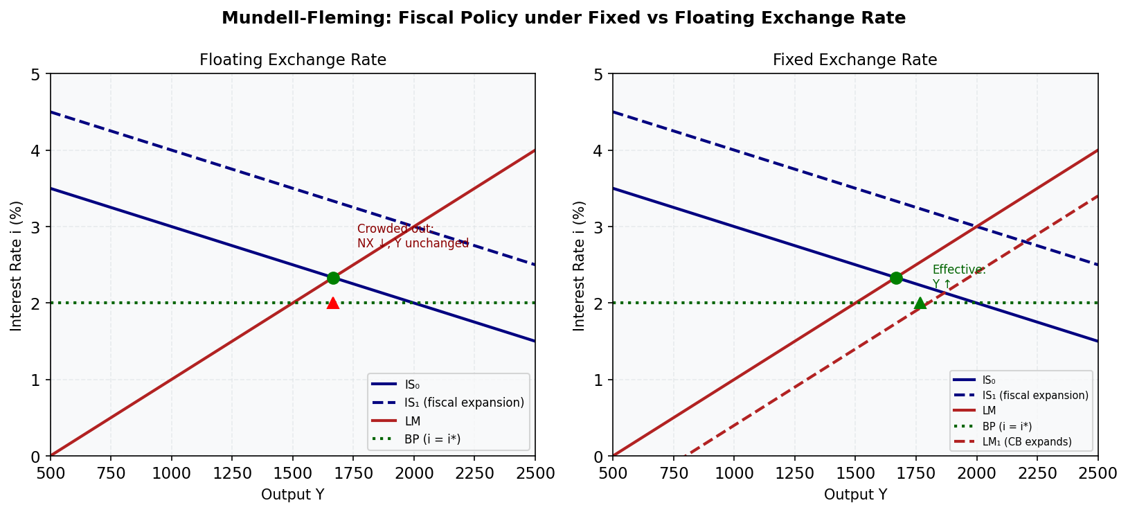
Figure 8: Mundell-Fleming. Under a floating exchange rate (left), fiscal expansion is crowded out via currency appreciation. Under a fixed exchange rate (right), the central bank accommodates and fiscal policy is effective.
The Mundell-Fleming model extends the closed-economy IS-LM framework to an open economy with internationally mobile capital. It is the workhorse model for analysing monetary and fiscal policy in open economies.
Three building blocks:
1. IS* curve (goods market equilibrium)
In a closed economy: Y = C(Y−T) + I(i) + G
In an open economy, we add net exports:
where ε = real exchange rate (units of foreign goods per unit of domestic goods; a rise in ε means the domestic currency is more expensive — an appreciation). Net exports NX decrease in ε: when the AUD appreciates, Australian exports become more expensive abroad and imports cheaper → NX falls.
For a given price level, ε and the nominal exchange rate e move together. In the Mundell-Fleming model, we typically work in Y-ε space (output vs. exchange rate). The IS* curve is negatively sloped: as ε rises (appreciation), NX falls, reducing aggregate demand and equilibrium Y.
2. LM* curve (money market equilibrium)
For a small open economy with perfect capital mobility, the domestic interest rate i is pinned at the world rate i*:
With i fixed at i*$, the LM* condition M/P = L(Y, i*) uniquely determines Y. The LM* curve is vertical* in (Y, ε) space — output is determined solely by the money supply and the world interest rate, regardless of the exchange rate.
3. Interest parity / BP = 0 curve
With perfect capital mobility, capital flows instantly to equate returns: i = i* + expected depreciation. In the short-run Mundell-Fleming model, exchange rate expectations are static, so the BP = 0 condition reduces to i = i*, already embedded in the LM*.
Small open economy assumption. Australia is a price-taker in world capital markets: it cannot influence i*. The RBA's cash rate can deviate temporarily from i*, but capital flows quickly restore parity.
Key notation: - Y = national output/income - ε = real exchange rate (higher = more appreciated) - i = domestic interest rate; i* = world interest rate - C = consumption; I = investment; G = government spending; NX = net exports - M/P = real money supply; L(Y, i) = money demand - IS* slopes down in (Y, ε) space; LM* is vertical in (Y, ε) space
Worked Example
Question: Derive the IS* curve algebraically and show it is negatively sloped in (Y, ε) space.
Assume linear functional forms:
- Consumption: C = 100 + 0.8(Y − T), with T = 50
- Investment: I = 200 − 500i (but i = i* = 0.05 is fixed, so I = 200 − 500×0.05 = 175)
- Government spending: G = 150
- Net exports: NX = 300 − 100ε
Step 1 — Substitute into the goods market equilibrium:
Step 2 — Expand consumption:
Step 3 — Collect Y terms:
Step 4 — Solve for Y (the IS* curve):
Interpretation: The IS* curve has slope dY/dε = −500. A 1-unit rise in the real exchange rate (appreciation) reduces equilibrium output by 500 units through the NX channel. This confirms the IS* curve is negatively sloped in (Y, ε) space.
Step 5 — Find the LM* equilibrium output:
Suppose M/P = 230 and money demand is L(Y, i*) = 0.1Y − 200i* = 0.1Y − 200×0.05 = 0.1Y − 10.
Setting M/P = L(Y, i*): 230 = 0.1Y − 10 → 0.1Y = 240 → Y* = 2,400
Step 6 — Find equilibrium ε:
From IS*: 2,400 = 3,425 − 500ε → 500ε = 3,425 − 2,400 = 1,025 → ε = 2.05
Equilibrium: Y* = 2,400, ε* = 2.05. A real exchange rate of 2.05 means domestic goods are relatively expensive; the current account is in surplus (NX = 300 − 100×2.05 = 300 − 205 = +95). The IS* and LM* intersection confirms goods and money markets clear simultaneously at i = i*.
Common Misconception
Misconception: "The LM* curve slopes upward in the Mundell-Fleming model, just like in the closed-economy IS-LM."
Correction: In the closed-economy IS-LM, the LM curve is plotted in (Y, i) space and slopes upward because higher Y raises money demand, requiring higher i for equilibrium. In the Mundell-Fleming model, the LM* curve is plotted in (Y, ε) space (not Y-i space). Because the interest rate is pinned at i* by perfect capital mobility, the exchange rate replaces the interest rate on the vertical axis. With i fixed, M/P = L(Y, i*) pins Y directly — so the LM* curve is vertical in (Y, ε) space. The exchange rate adjusts to clear the goods market (IS*), not the money market.
Practice Prompts
- Conceptual: Explain why the IS* curve is negatively sloped in (Y, ε) space while the LM* curve is vertical. What does each curve represent?
→ Answer: The IS* curve represents goods market equilibrium. A rise in ε (appreciation) reduces NX → reduces aggregate demand → reduces equilibrium Y. So Y and ε are negatively related along IS*. The LM* curve represents money market equilibrium under the constraint i = i* (perfect capital mobility). With i pinned, the equation M/P = L(Y, i*) determines Y uniquely — there is only one Y consistent with money market equilibrium regardless of ε. Hence LM* is vertical.
- Numerical: Using the IS* derived above (Y = 3,425 − 500ε), calculate equilibrium Y if ε = 2.5. Then suppose government spending rises from G = 150 to G = 200: recalculate the new IS* equation and find the new equilibrium Y at ε = 2.5.
→ Answer: - Initial: Y = 3,425 − 500(2.5) = 3,425 − 1,250 = 2,175 - ΔG = +50, with multiplier effect on intercept: ΔY-intercept = ΔG/(1−MPC) = 50/0.2 = +250 - New IS*: Y = (3,425 + 250) − 500ε = 3,675 − 500ε - New Y at ε = 2.5: Y = 3,675 − 1,250 = 2,425
(Note: this is the goods-market effect only; the full Mundell-Fleming analysis under floating or fixed rates is covered in M20.L02–L03.)
- Application: Australia is typically modelled as a small open economy. What does this assumption imply for the relationship between the RBA's cash rate and the world interest rate i*?
→ Answer: As a small open economy with a floating exchange rate and open capital account, Australia is a price-taker in world capital markets. The small open economy assumption implies that Australia cannot persistently set its interest rate above or below i* without triggering capital flows that offset the policy. In practice, the RBA cash rate can deviate from i* temporarily (especially the US Federal Funds Rate) due to risk premia, inflation differentials, and delayed capital adjustment. But sustained deviations trigger exchange rate movements (AUD appreciation if RBA rate > i*; depreciation if below) that partially erode the policy's domestic demand effects.
Visual — The Mundell-Fleming IS–LM Diagram
Figure: In the Mundell-Fleming model, IS slopes downward in (Y, ε) space while LM is vertical. A rise in the exchange rate moves the economy up along IS and reduces output.*
Further Resources
- 📺 Open Economy Macroeconomics: The Mundell-Fleming Model — Academic Economics (45 min)
- 📺 Lecture 20: The Mundell-Fleming Model — MIT OCW — MIT OpenCourseWare (50 min)
- 📚 MIT OCW 14.02 Macroeconomics — Full lecture notes including Mundell-Fleming