Lesson M14.L01: The IS Curve: Goods Market Equilibrium
Module: The IS-LM Model Part I Level: intermediate Duration: 30 minutes Learning Objective: Derive the IS curve by tracing goods market equilibrium across different interest rates. Data as of: 2024 Provenance: OpenStax Macro 3e | MIT OCW 14.02 | RBA
Explanation
Key Diagram
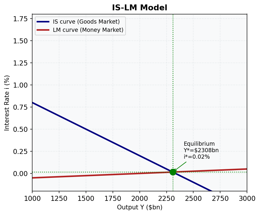
Figure 5: The IS-LM Model. The IS curve (goods market) and LM curve (money market) intersect at equilibrium output Y and interest rate i.
The IS curve maps all combinations of output (Y) and the interest rate (i) at which the goods market is in equilibrium (planned expenditure equals output). It is derived by embedding the interest-sensitive investment function into the Keynesian cross.
Setup. Introduce I = Ī − bi (from M13.L03) into the Keynesian cross:
Y = C + I + G + NX Y = (a + b_c(Y − T̄)) + (Ī − bi) + Ḡ + (X̄ − mY)
Note: to avoid symbol clash, let b_c = MPC and b_i = interest sensitivity of investment. In what follows b_c is written as b and the investment sensitivity as b_inv, consistent with standard notation where context distinguishes them.
Using b for MPC throughout and b_inv for interest sensitivity of investment:
Y(1 − b + m) = a − bT̄ + Ī − b_inv·i + Ḡ + X̄
Solving for Y:
To express as the IS curve, rearrange for i as a function of Y:
(1 − b + m)Y = a − bT̄ + Ī + Ḡ + X̄ − b_inv·i b_inv·i = a − bT̄ + Ī + Ḡ + X̄ − (1 − b + m)Y i = [a − bT̄ + Ī + Ḡ + X̄ − (1 − b + m)Y] / b_inv
Define autonomous spending A = a − bT̄ + Ī + Ḡ + X̄:
Slope: The IS curve has a negative slope in (Y, i) space: di/dY = −(1 − b + m)/b_inv < 0.
Steepness: The curve is steeper when (1 − b + m)/b_inv is large — i.e., when b (MPC) is lower (more leakage to saving), m is higher (more import leakage), or b_inv is smaller (investment less responsive to interest rates).
Shifts: IS shifts right (more output at given i) when G↑, T̄↓, X̄↑, or a↑ (any rise in autonomous spending). IS shifts left when G↓, T̄↑, X̄↓.
Worked Example
Parameters: a = 200, b = 0.8 (MPC), T̄ = 100, Ī = 150, Ḡ = 250, X̄ = 180, m = 0.1, b_inv = 500 (interest sensitivity of investment).
Step 1 — Compute autonomous spending A:
A = a − bT̄ + Ī + Ḡ + X̄ = 200 − (0.8)(100) + 150 + 250 + 180 = 200 − 80 + 150 + 250 + 180 = 700
Step 2 — Write the IS curve (Y as function of i):
Y = (700 − 500i) / (1 − 0.8 + 0.1) = (700 − 500i) / 0.3
Step 3 — Find Y* when i = 0.04 (4%):
Y = (700 − 500 × 0.04) / 0.3 = (700 − 20) / 0.3 = 680 / 0.3 = $2,267bn
Step 4 — Find Y* when i = 0.07 (7%):
Y = (700 − 500 × 0.07) / 0.3 = (700 − 35) / 0.3 = 665 / 0.3 = $2,217bn
Step 5 — Compute the IS slope (i as function of Y):
i = 700/500 − (0.3/500)Y = 1.4 − 0.0006Y
A 1-unit increase in Y reduces i by 0.0006 percentage points; equivalently, a 1 percentage point rise in i reduces Y by 1/0.0006 ≈ $1,667bn (the horizontal shift in Y for a given Δi).
Common Misconception
Misconception: The IS curve slopes downward because lower interest rates directly stimulate consumer spending on goods.
Correction: In the standard model, the interest rate affects the goods market through investment, not directly through consumption. Lower i → higher I (via I = Ī − b_inv·i) → higher autonomous spending → higher equilibrium Y via the multiplier. The consumption function C = a + b(Y − T̄) responds to income, not directly to i (in the basic model). The IS curve's negative slope is entirely the investment-multiplier channel.
Practice Prompts
-
List three exogenous shocks that would shift the IS curve to the right, and explain the channel through which each operates. → Answer: (1) Government spending increase (ΔḠ > 0): Raises autonomous spending directly; at any given interest rate, equilibrium Y is higher. (2) Tax cut (ΔT̄ < 0): Raises household disposable income, boosting consumption (ΔC = b × |ΔT̄|), shifting IS right. (3) Export boom (ΔX̄ > 0): Raises autonomous net exports, increasing aggregate expenditure at every i; Y* rises via multiplier. All three increase A, the numerator of the IS equation, shifting IS rightward.
-
Using b = 0.8, m = 0.15, T̄ = 150, a = 180, Ī = 200, Ḡ = 220, X̄ = 160, b_inv = 400, compute equilibrium Y when i = 0.05 (5%) and when i = 0.10 (10%). What is ΔY from the interest rate rise? → Answer:
- A = 180 − (0.8)(150) + 200 + 220 + 160 = 180 − 120 + 200 + 220 + 160 = 640
- Denominator: 1 − 0.8 + 0.15 = 0.35
- At i = 0.05: Y = (640 − 400 × 0.05)/0.35 = (640 − 20)/0.35 = 620/0.35 = $1,771bn
- At i = 0.10: Y = (640 − 400 × 0.10)/0.35 = (640 − 40)/0.35 = 600/0.35 = $1,714bn
-
ΔY = 1,714 − 1,771 = −$57bn (a 5pp interest rate rise reduces output by $57bn)
-
During 2022–2023, the RBA raised the cash rate from 0.10% to 4.35% — a rise of 425 basis points. Using the IS framework, explain through which channels this would have reduced Australian GDP, and why the effect may have been larger than a simple model predicts. → Answer: Via the IS channel: higher i reduces investment (I = Ī − b_inv·i falls), shifting the economy up the IS curve (or equivalently, reducing autonomous expenditure, lowering Y via the multiplier). Additional channels beyond the basic model: (1) Mortgage cash flow: Australia has a high proportion of variable-rate mortgages; rate rises rapidly increased mortgage repayments, directly reducing household disposable income and consumption — equivalent to a tax increase. (2) Consumer confidence: Rate rises signalled future tightening, reducing autonomous consumption a. (3) Housing investment collapse:* Rising rates decimated new housing construction (dwelling investment fell ~15% in 2023). These amplifying channels made the RBA's tightening more powerful than the basic model's investment-only channel implies.
Visual — The IS Curve: Movements and Shifts
Figure: The IS curve is downward sloping because higher interest rates reduce investment and equilibrium output. A fiscal expansion raises autonomous demand and shifts the whole IS curve to the right.
Further Resources
- 📺 Macroeconomics: The IS Curve — Economics in Many Lessons (15 min)
- 📺 Macroeconomics: The IS-LM Model — Economics in Many Lessons (15 min)
- 📚 RBA — Monetary Policy Explainer — Goods market equilibrium and how the IS curve underpins RBA modelling